Tiny transformers for population genetic inference

The self-attention mechanism works quite well for recombination rate classification

Introduction

Representing genetic variation with PNGs

Take a look at the two images below. These images are of shape \((H = 64, W = 36)\) — each row represents a human haplotype, and each column represents a single-nucleotide polymorphism (SNP). Each “pixel” location \(H_i, W_j\) can take a value of \(0\) (meaning haplotype \(i\) possesses the ancestral allele at site \(j\)) or \(1\) (meaning it possesses the derived allele).

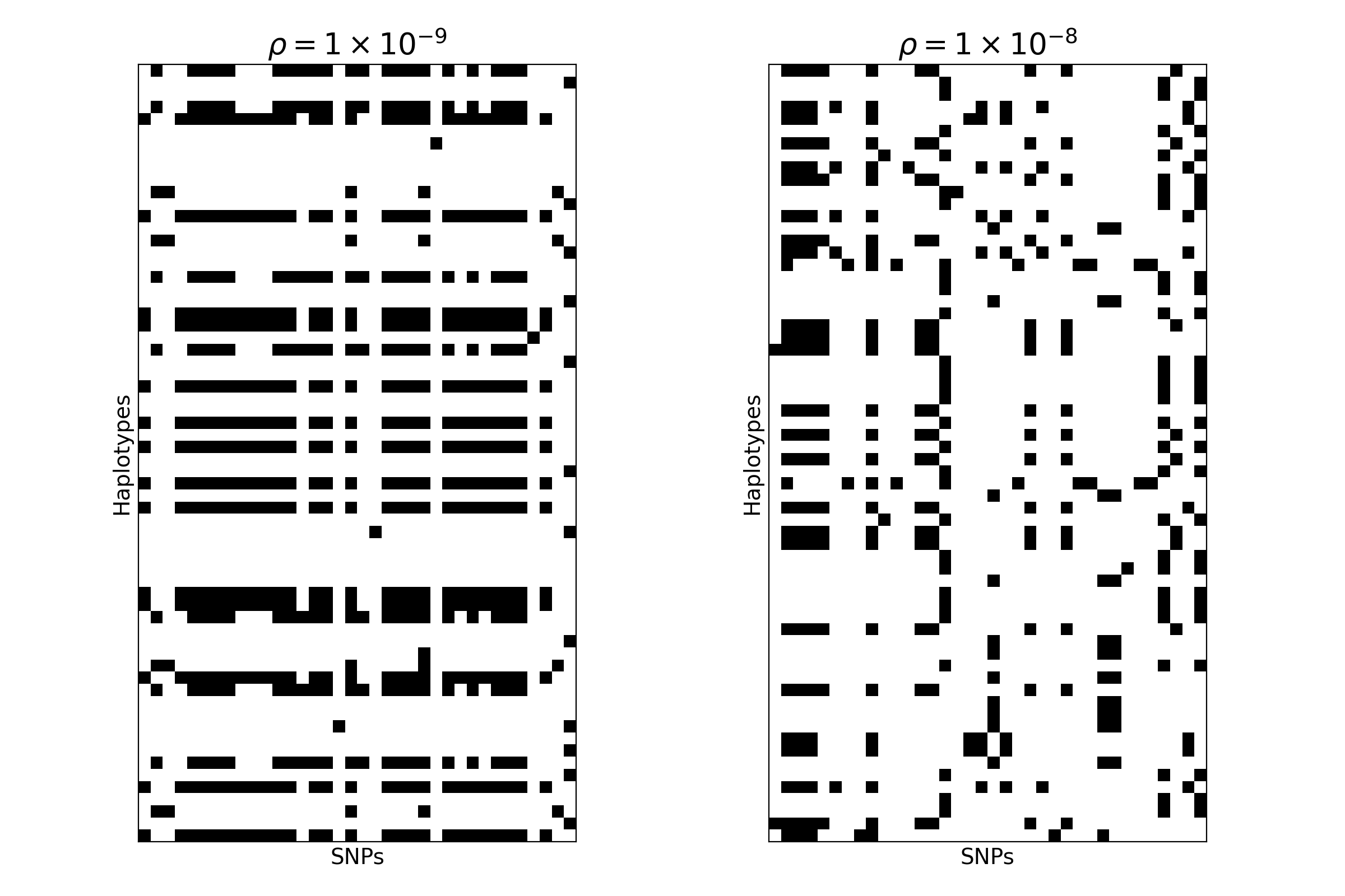
Both images were simulated using a backwards-in-time simulation engine called msprime, and each image represents the genetic variation present in collection of \(H = 64\) haplotypes sampled at \(W = 36\) consecutive SNPs. The genomes in the first image were simulated from a demographic model in the stdpopsim catalog¹, assuming a recombination rate \(\rho = 10^{-9}\). The genomes in the second image were simulated from the same demographic model, but assuming \(\rho = 10^{-8}\).

Classifying images of genetic variation with machine learning

By eye, we might be able to tell a difference between the two images, but what if we wanted to classify tens or hundreds of thousands of them? This example is totally contrived, but it represents an important kind of inference challenge in population genetics: distinguishing between the patterns of genetic variation observed in different regions of the genome. For example, we might want to discriminate between regions of the genome undergoing positive or negative selection and those evolving neutrally or near-neutrally. Although numerous statistical methods exist for doing this kind of inference, machine learning methods may be particularly well-suited to the task.

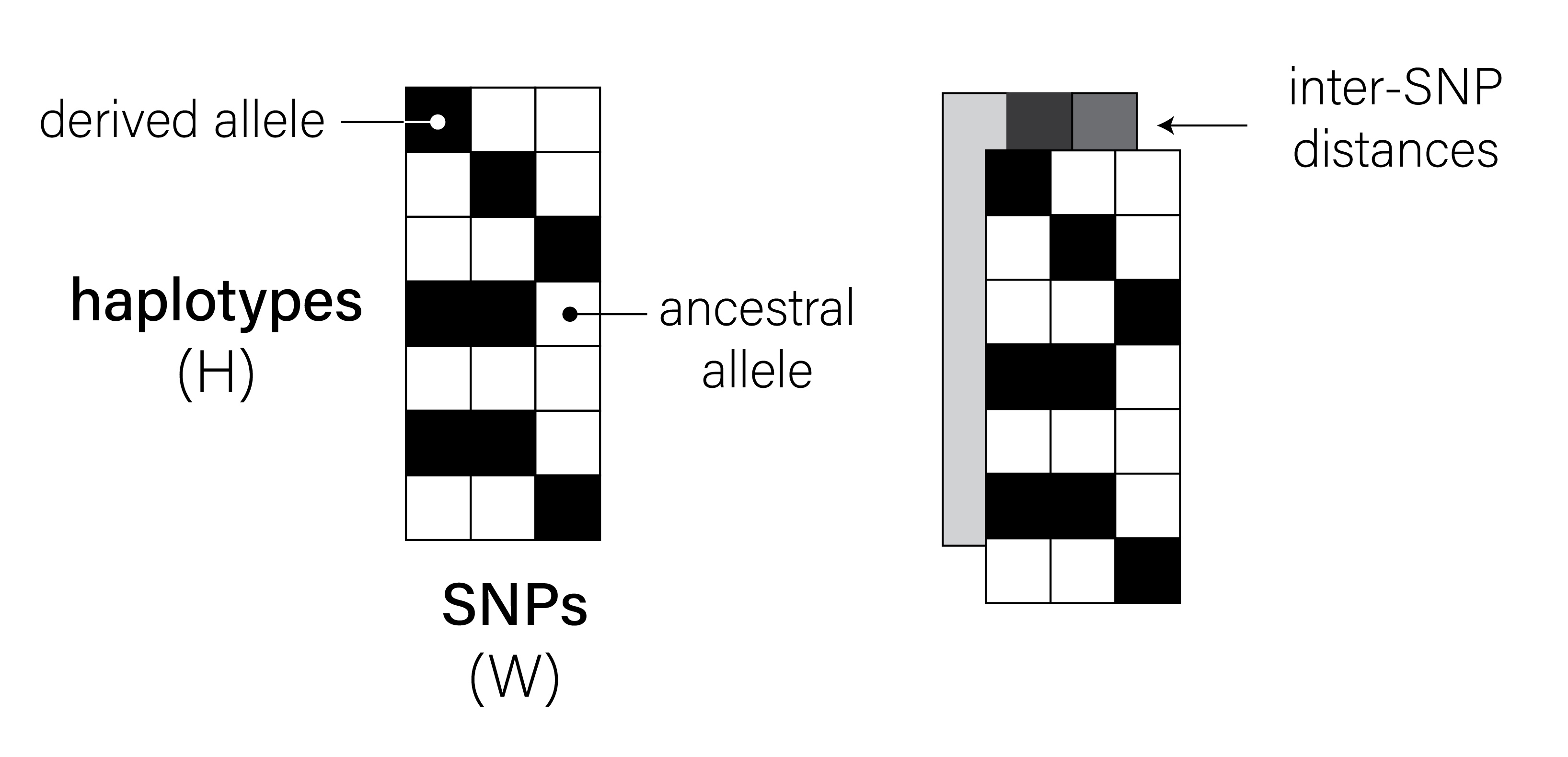
Machine learning approaches — in particular, convolutional neural networks (CNNs) — have proven “unreasonably effective”² for population genetic inference. CNNs can be trained to detect population genetic phenomena (e.g., selection³, adaptive admixture⁴, incomplete lineage sorting⁵) and predict various summary statistics (e.g., recombination rate) by ingesting lots of labeled training data. These training data often comprise 1- or 2-channel “images” of haplotypes in genomic windows of a defined SNP length (see Figure 1), much like the ones shown above.

Figure 1: Learning from images of haplotypes. We can represent genomic regions as one- or two-channel “images” in which rows correspond to haplotypes and columns to SNPs. The first channel typically encodes derived alleles as \(1\)s and ancestral alleles as \(0\)s, while the second channel can encode either absolute genomic positions or inter-SNP distances. In the absence of phased haplotype data, the first channel can also represent diploid genotypes as \(0\) (homozygous for the ancestral allele), \(0.5\) (heterozygous), and \(1\) (homozygous for the derived allele).

Images of human haplotypes aren’t like images of cats

Exchangability and permutation-invariance

Unlike images of cats, dogs, or handwritten digits, these images of human genetic variation are “row-invariant.” In other words, the information in the image is exactly the same regardless of how you permute the haplotypes. If you were to shuffle the rows of an image of a cat, on the other hand, that image would look dramatically different, and the spatial correlations between pixels would be totally broken.

The order of haplotypes in an image might matter if the haplotypes are derived from two or more highly structured populations, or if we’ve introduced structure into the image by e.g., sorting haplotypes by genetic similarity. In general, though, we’d like to develop machine learning methods that are agnostic to both haplotype order and number.

To enable permutation-invariant population genetic inference on images of human haplotypes, Chan et al. developed the defiNETti architecture (details in Note 1).

Note 1: The defiNETti architecture: a powerful, yet conceptually simple, machine learning approach designed for images of genetic variation

First, a series of strided 1D convolutions are applied to an input image of genetic variation (optionally followed by activation functions and pooling) to create high-dimensional feature maps and reduce the width of the input image. These 1D convolutions can presumably capture “interesting” features, like linkage disequilibrium between nearby SNPs, as well as build higher-level combinations of those features. After the convolutional layers we’re left with a batch of tensors of shape \((B, D, H, W')\), where \(B\) is the batch size, \(D\) is the number of feature maps produced by the convolutional operations, \(H\) is the original height of the image (i.e., the number of haplotypes) and \(W'\) is the width of the image after strided convolutions and pooling operations are taken into account. 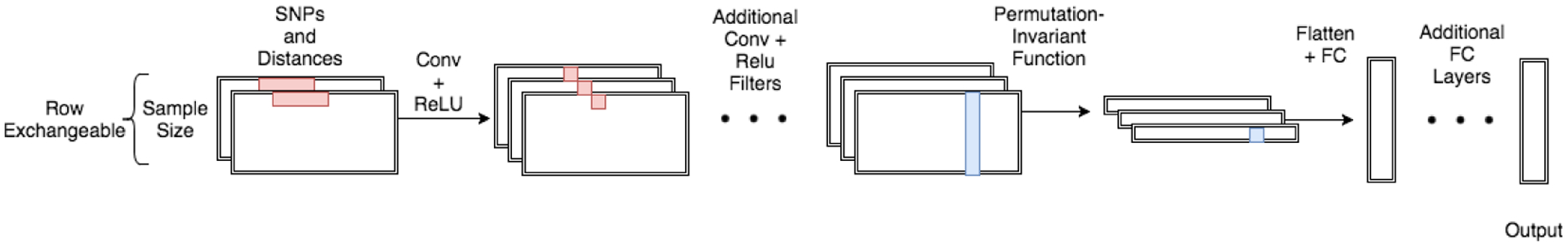To make the model agnostic to both the order and number of haplotypes in the input image, a “permutation-invariant” aggregation operation is then applied along the \(H\) dimension (typically, max or mean). Then, the resulting tensor of shape \((B, D, 1, W)\) can be flattened and passed through a series of fully-connected layers and a final classification head.

From Chan et al. (2019) Advances in NeurIPS.

Chan et al. demonstrate that their approach is highly effective for a number of population genetics inference tasks, and outperforms established statistical methods for e.g., the detection of recombination hotspots. In addition to being permutation-invariant, the aggregation operation applied before its fully-connected layers means that defiNETti is also (mostly) agnostic to sample size. Even if defiNETti is trained on images of height \(H = 512\), it is insensitive to the sizes of images at test time, working quite well even when images contain as few as 64 haplotypes. In the population genetics setting, permutation-invariance and sample size indifference are extremely attractive properties of a machine learning method. For example, we might want to train a machine learning model using data from one cohort (say, a subpopulation of the Thousand Genomes consortium), and test that model on haplotypes sampled from another cohort with fewer or more samples.

Transformers as permutation-invariant architectures

Although the defiNETti approach demonstrated that permutation-invariant CNNs are powerful, lightweight tools for population genetic inference, other architectures may be even better. For example, the transformer architecture, and the self-attention mechanism in particular, is a natural choice for embedding images of human genetic variation. To my knowledge, though, transformers are relatively unexplored in the population genetics space.

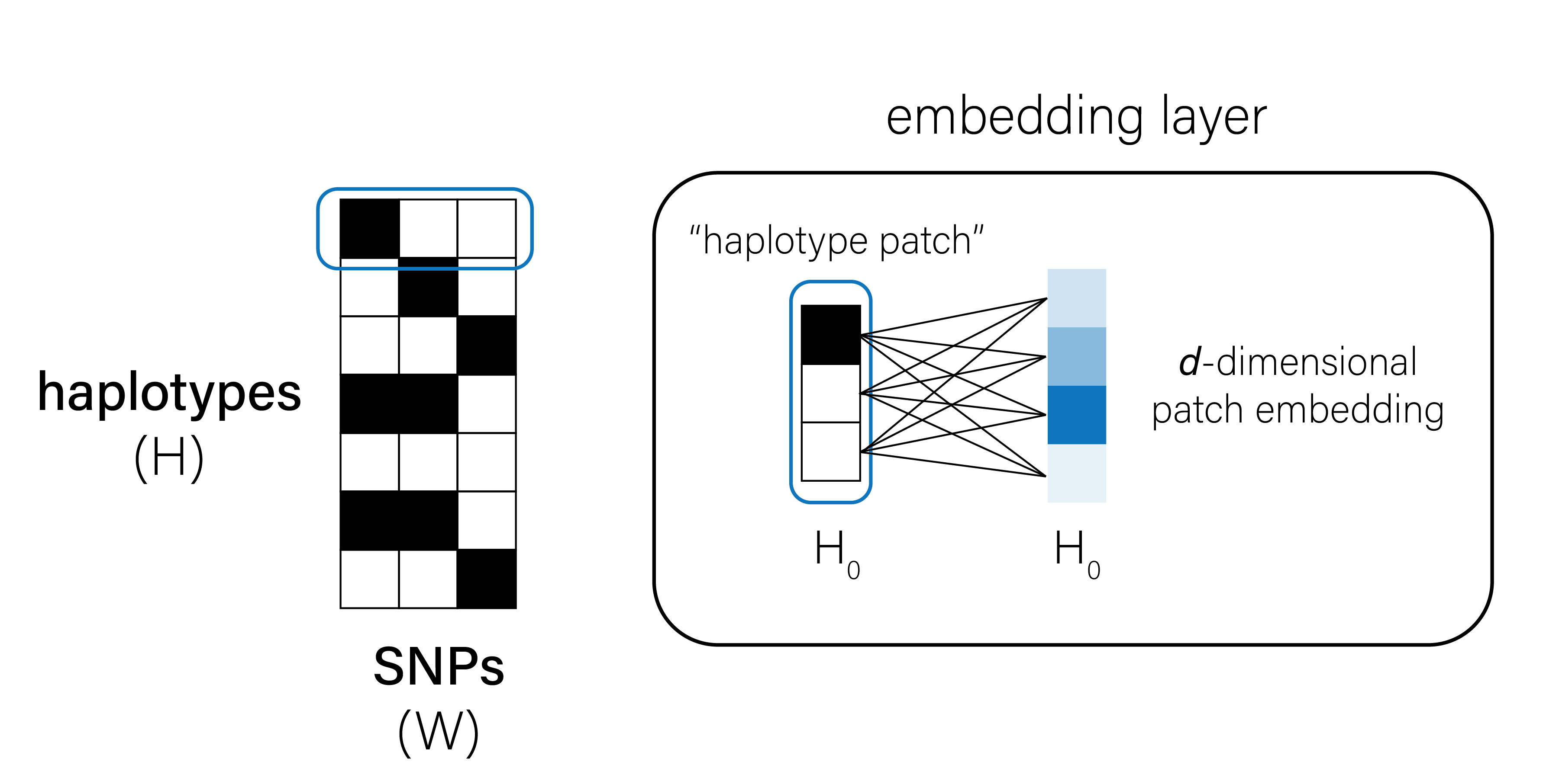
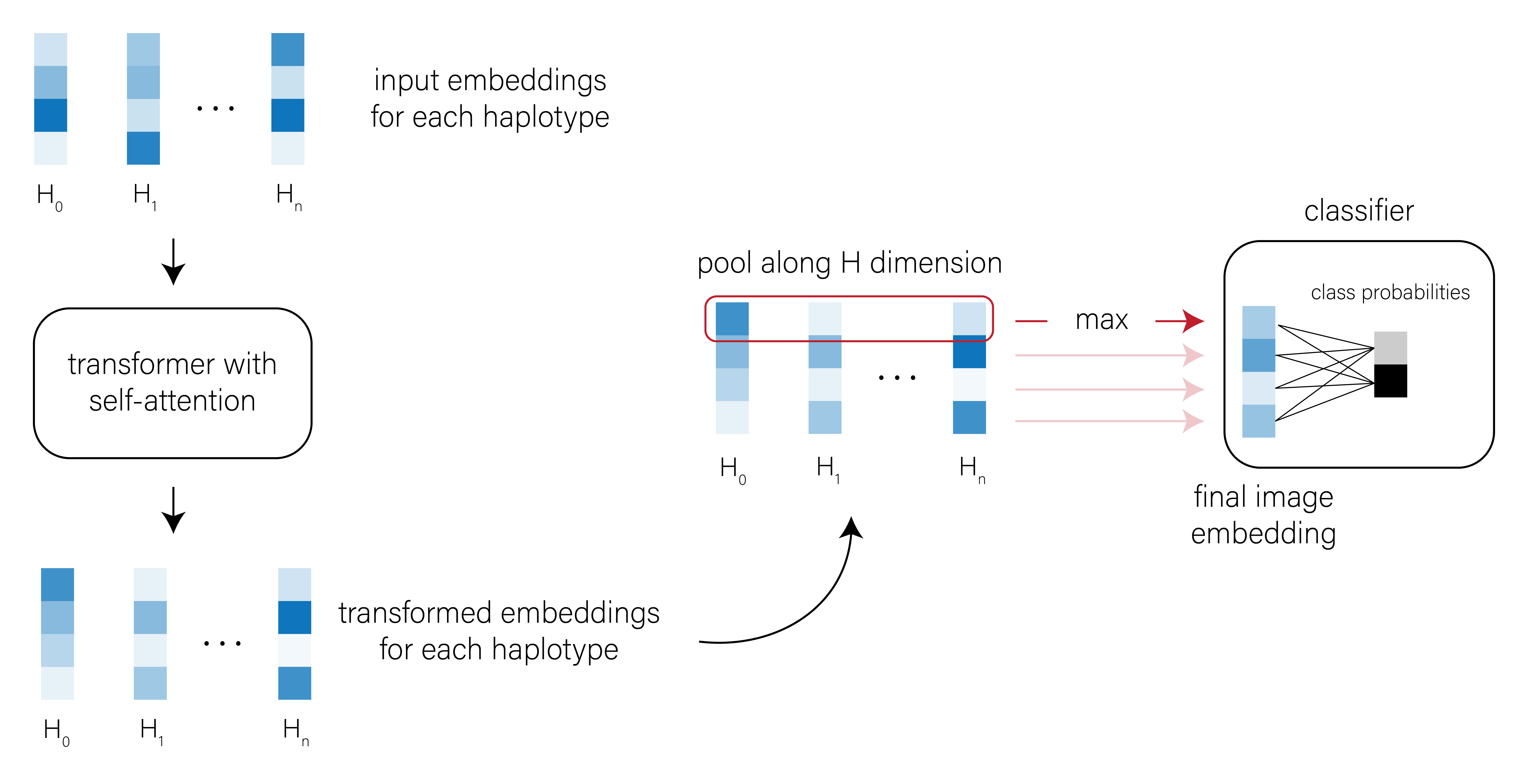
In the parlance of the vision transformer (ViT)⁶, we can treat input images of genetic variation as collections of “haplotype patches.” Each patch \(P\) is shape \((1, W)\), where \(W\) is the number of SNPs and \(P \in \{0, 1\}\). We first embed each patch in a new, \(d\)-dimensional feature space using a single fully-connected layer (Figure 2).

Figure 2: Tokenizing haplotype images. Given an image of genetic variation, we embed every haplotype “patch” into a new \(d\)-dimensional embedding space using a single fully-connected layer (essentially, just a linear transformation of the \(0\)s and \(1\)s each haplotype possesses at the \(W\) SNPs.)

I won’t spend much time on the details here, but the basic conceit of self-attention is that the embedding of each patch is compared to the embedding of every other patch, and the weights associated with these pairwise comparisons can be tuned to capture the important relationships between patches. The transformer outputs an updated set of haplotype patch embeddings that should reflect these inter-haplotype relationships (Figure 3).

For a great overview of the transformer architecture, including the building blocks of self-attention, check out the Illustrated Transformer.

Figure 3: Applying transformers to haplotype images. For a given image, we pass the haplotype patch embeddings from Figure 2 to a transformer with self-attention. A transformer module (details in Note 2) outputs a new, “updated” set of haplotype patch embeddings. We can create a final image embedding by simply aggregating across haplotype patches at each dimension \(d_i\) of the embedding space, then add a fully-connected layer on top of that final image embedding for classification purposes. Alternatively, we could include a special [CLS] classification token when training the transformer and use its output embedding for classification tasks.

Note 2: The transformer module in more detail

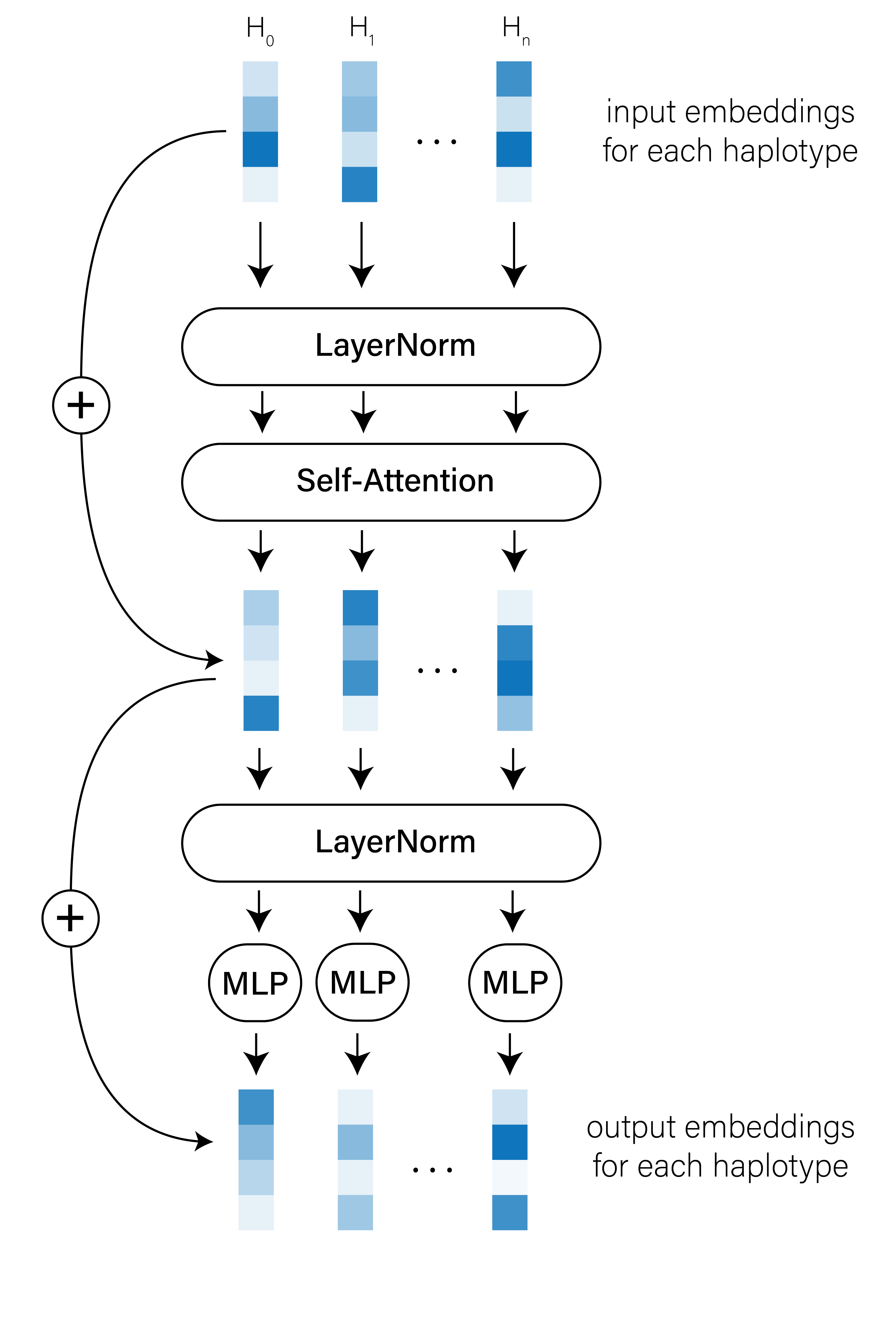
Each transformer “module” comprises multiple layers of normalization, residual connections and multi-layer-perceptrons (MLPs). First, the input embeddings are normalized using LayerNorm. Next, the normalized embeddings are fed into a multi-headed self-attention block. A residual skip connection adds the output of that self-attention block to the original input embeddings. Those embeddings are normalized again, and then each haplotype (token) embedding is passed through a fully-connected feed-forward (FCFF) network with one hidden layer (in these experiments, the FCFF network has a hidden layer of size \(2d\), where \(d\) is the dimensionality of the input embeddings). A final residual connection sums the output of the FCFF network and the output of the first skip connection to produce the final haplotype embeddings.

The self-attention mechanism is inherently invariant to the order of the patch embeddings, though we could introduce learned positional/rotary embeddings into our model if their order does matter. It can also be applied to images with any number of haplotypes (assuming our CPU/GPU hardware can handle the sequence length).

So, how well do transformers work for population genetic inference?

Materials and Methods

Let’s compare a simple transformer model to a simple implementation of the defiNETti architecture. I’ve included pytorch code for replicating the two models below.

Architectural details

CNN model architectures were adapted from Chan et al. (defiNETti) and Wang et al. (2021). Convolutional operations used a kernel of shape (1, 5), stride of (1, 1), and no zero-padding. All convolutional operations were followed by ReLU activations. In the Wang et al. architecture, convolutional operations were further followed by MaxPool with a stride and kernel of (1, 2). The first convolutional layer always outputs a feature map with 32 channels, and feature maps increased in dimension by a factor of 2 with each subsequent convolutional layer. I used max as the permutation-invariant function (to collapse along the height dimension) in all cases; empirically, I found that max outperformed mean as an aggregation function. After applying the permutation-invariant function, feature maps were flattened and passed to two fully-connected layers of 128 dimensions each, with ReLU activations after each.

Our transformer model architecture follows the same general structure as in the Vision Transformer (ViT) paper — see Equations 1-4 in the ViT preprint (or the code samples below) for details. Briefly, we embedded haplotype patches using a single fully-connected layer with 128 dimensions and passed the resulting tensor of patch embeddings to a single multi-headed self-attention block with 8 heads, LayerNorm, a multi-layer perceptron (MLP) and residual connections.

CNN model architecture

model type	kernel size	stride	max-pool	convolutional layers	fully-connected dimension	trainable params (hotspot task)	trainable params (rate task)
CNN (defiNETti)	5	1	False	2	128	256,770	256,899
CNN (Wang et al.)	5	1	True	2	128	76,546	76,675

Transformer architecture

model type	depth	hidden size	MLP size	heads	trainable params (hotspot task)	trainable params (rate task)
Transformer	1	128	256	8	137,603	137,732

All models were trained with the Adam optimizer. As in Chan et al., we used the following learning rate schedule: \(10^{-3} \times 0.9^{\frac{m}{I}}\), where \(m\) is the current minibatch and \(I\) is the total number of training iterations.

“Tokenizer” for embedding haplotype patches

from torch import nn

class HaplotypeTokenizer(nn.Module):

    def __init__(
        self,
        input_channels: int = 1,
        input_width: int = 36,
        hidden_size: int = 128,
    ):
        super().__init__()

        self.input_dim = input_channels * input_width
        self.hidden_size = hidden_size
        # simple linear projection
        self.proj = torch.nn.Linear(self.input_dim, hidden_size)

    def forward(self, x):
        # shape should be (B, C, H, W) where H is the number
        # of haplotypes and W is the number of SNPs
        B, C, H, W = x.shape
        # permute to (B, H, C, W)
        x = x.permute(0, 2, 1, 3)
        # then, flatten each "patch" of C * W such that
        # each patch is 1D and size (C * W).
        x = x.reshape(B, H, -1)
        # embed "patches" of size (C * W, effectively a 1d
        # array equivalent to the number of SNPs)
        tokens = self.proj(x)
        return tokens

A simple transformer model with self-attention

class Transformer(nn.Module):

    def __init__(
        self,
        embed_dim: int = 128,
        num_heads: int = 1,
        mlp_hidden_dim_ratio: int = 2,
    ):
        super().__init__()

        self.attn = nn.MultiheadAttention(
            embed_dim,
            num_heads,
            batch_first=True,
        )
        self.norm = nn.LayerNorm(embed_dim)

        self.mlp = nn.Sequential(
            nn.Linear(embed_dim, embed_dim * mlp_hidden_dim_ratio),
            nn.GELU(),
            nn.Linear(embed_dim * mlp_hidden_dim_ratio, embed_dim),
        )

    def forward(self, x):
        # layernorm initial embeddings
        x_norm = self.norm(x)
        # self-attention on normalized embeddings
        attn_out, _ = self.attn(x_norm, x_norm, x_norm)  
        # residual connection + layernorm
        x = self.norm(x + attn_out)
        # mlp on each haplotype token
        x_mlp = self.mlp(x)
        # final residual connection + layernorm
        return self.norm(x + x_mlp)


class TinyTransformer(torch.nn.Module):
    def __init__(
        self,
        width: int = 36,
        in_channels: int = 1,
        num_heads: int = 1,
        hidden_size: int = 128,
        num_classes: int = 2,
        depth: int = 1,
        mlp_ratio: int = 2,
        agg: str = "max",
    ):
        super().__init__()

        self.hidden_size = hidden_size
        self.norm = nn.LayerNorm(hidden_size)
        self.agg = agg

        # we use a "custom" tokenizer that takes
        # patches of size (C * W), where W is the
        # number of SNPs
        
        self.tokenizer = ColumnTokenizer(
            input_channels=in_channels,
            input_width=width,
            hidden_size=hidden_size,
        )

        self.attention = nn.Sequential(
            *[
                Transformer(
                    embed_dim=hidden_size,
                    num_heads=num_heads,
                    mlp_hidden_dim_ratio=mlp_ratio,
                )
                for _ in range(depth)
            ]
        )

        # linear classifier head
        self.classifier = torch.nn.Linear(
            hidden_size,
            num_classes,
        )

    def forward(self, x):
        B, C, H, W = x.shape
        x = self.tokenizer(x)  # (B, H, hidden_size)
        # pass through transformer encoder
        x = self.attention(x)
        if self.agg == "max":
            cls_output = torch.amax(x, dim=1)
        elif self.agg == "mean":
            cls_output = torch.mean(x, dim=1)
        logits = self.classifier(cls_output)

        return logits

The defiNETti architecture

class DeFinetti(nn.Module):

    def __init__(
        self,
        *,
        in_channels: int,
        kernel: Union[int, Tuple[int]] = (1, 5),
        hidden_dims: List[int] = [32, 64],
        agg: str = "max",
        width: int = 36,
        num_classes: int = 2,
        fc_dim: int = 128,
        padding: int = 0,
        stride: int = 1,
        pool: bool = False,
    ) -> None:

        super(DeFinetti, self).__init__()

        self.agg = agg
        self.width = width

        _stride = (1, stride)
        _padding = (0, padding)

        out_W = width

        conv = []
        for h_dim in hidden_dims:
            # initialize convolutional block
            block = [
                nn.Conv2d(
                    in_channels,
                    h_dim,
                    kernel_size=kernel,
                    stride=_stride,
                    padding=_padding,
                ),
                nn.ReLU(),
            ]
            if pool:
                block.append(
                    nn.MaxPool2d(
                        kernel_size=(1, 2),
                        stride=(1, 2),
                    ),
                )
            
            out_W = (
                math.floor((out_W - kernel[1] + (2 * (padding))) / _stride[1]) + 1
            )

            # account for max pooling
            if pool:
                out_W //= 2
            in_channels = h_dim
            conv.extend(block)

        self.conv = nn.Sequential(*conv)
        self.fc = nn.Sequential(
            nn.Linear(hidden_dims[-1] * out_W, fc_dim),
            nn.ReLU(),
            nn.Linear(fc_dim, fc_dim),
            nn.ReLU(),
        )
        # two projection layers with batchnorm
        self.project = nn.Sequential(
            nn.Linear(fc_dim, num_classes),
        )
        self.flatten = nn.Flatten()

    def forward(self, x):
        x = self.conv(x)
        # take the average across haplotypes
        if self.agg == "mean":
            x = torch.mean(x, dim=2)
        elif self.agg == "max":
            x = torch.amax(x, dim=2)
        elif self.agg is None:
            pass
        # flatten, but ignore batch
        x = self.flatten(x)
        encoded = self.fc(x)
        projection = self.project(encoded)

        return projection

Training datasets and classification tasks

I compared the performance of CNNs and transformers on two simple classification tasks.

Recombination hotspot detection

The first task was adapted from Chan et al. Training data belonged to one of two classes: regions that either contained or did not contain a recombination hotspot. All regions were simulated using a simple msprime demographic model and an msprime recombination RateMap object as follows:

Simulating recombination hotspots

import msprime
import numpy as np

rng = np.random.default_rng(42)

# interval length
L = 25_000
# hotspot length
HOTSPOT_L = 2_000

# define background recomb rate
background = rng.uniform(1e-8, 1.5e-8)

class_label = rng.choice(2)
heat = 1 if class_label == 0 else rng.uniform(10, 100)

# starts and ends of the hotspot given length of simulated inderval
hs_s, hs_e = (
    (L - HOTSPOT_L) / 2,
    (L + HOTSPOT_L) / 2,
)
rho_map = msprime.RateMap(
    position=[
        0,
        hs_s,
        hs_e,
        L,
    ],
    rate=[background, background * heat, background],
)

seed = rng.integers(0, 2**32)
ts = msprime.simulate(
    sample_size=200,
    Ne=1e4,
    recombination_map=rho_map,
    mutation_rate=1.1e-8,
    random_seed=seed,
)

In all rate maps, \(\rho_{bg} \sim \mathcal{U}\{1 \times 10^{-8}, 1.5 \times 10^{-8}\}\).

Regions with recombination hotspots

left	right	mid	span	rate
0	11,500	5,750	11,500	\(\rho_{bg}\)
11,500	13,500	12,500	2,000	\(\rho_{bg} \times \mathcal{U}\{10, 100\}\)
13,500	25,000	19,250	11,500	\(\rho_{bg}\)

Regions without recombination hotspots

left	right	mid	span	rate
0	25,000	12,500	25,000	\(\rho_{bg}\)

Recombination rate classification

In the second task, training data belonged to one of three classes: regions with one of three different recombination rates (\(10^{-7}\), \(10^{-8}\), or \(10^{-9}\)). All regions were simulated using a CEU population from the OutOfAfrica_3G09 model⁷ in the stdpopsim catalog.

Simulating variable recombination rates

import stdpopsim

# choose species and model
species = stdpopsim.get_species("HomSap")
demography = species.get_demographic_model("OutOfAfrica_3G09")
RHO = [1e-9, 1e-8, 1e-7]

contigs = [
    species.get_contig(
        length=50_000,
        recombination_rate=r,
        mutation_rate=2.35e-8,
    )
    for r in RHO
]

# msprime by default
engine = stdpopsim.get_default_engine()

samples_per_population = [0, 0, 0]
# use a CEU population
samples_per_population[1] = n_smps
samples = dict(
    zip(
        ["YRI", "CEU", "CHB"],
        samples_per_population,
    )
)

class_label = rng.choice(3)

ts = engine.simulate(
    demography,
    contig=contigs[class_label],
    samples=samples,
)

Simulation “on-the-fly”

Rather than train these models with a fixed dataset of \(N\) images, I simulated training examples “on the fly” as described in Chan et al. In each training iteration, I simulated a fresh minibatch of 256 haplotype images of shape \((1, 200, 36)\) — with approximately equal contribution from each class — passed the minibatch through the model, and updated the model weights using cross-entropy loss. As the models never saw the same image twice during training, there was no need to run them on a “held out” validation or test set. Models were trained for 1,000 iterations (one minibatch per iteration); therefore, each model saw a total of 25,600 unique images during training. I used random seeds to ensure that each model saw the same 25,600 images during training.

Results

Transformer models outperform CNNs for recombination rate classification

Overall, the transformer exhibits higher accuracy than the CNNs on the recombination rate classification task (Figure 4).

(a)

(b)

(c)

Figure 4

Transformer models slightly outperform CNNs for recombination hotspot detection

Transformer and CNN performance is more similar on the recombination hotspot detection task (Figure 5), though the former still exhibits better accuracy.

(a)

(b)

Figure 5

Future work

This was a very simple experiment, and involved very little hyper-parameter or model tuning. At the very least, it suggests that simple transformers with self-attention are useful architectures for population genetics inference. There are many ways to investigate their utility further.

• test models on more complex and realistic classification tasks
• tweak both CNNs and transformers to find optimal hyper-parameters
  • perhaps we could engineer CNNs to have comparable performance?
• compare performance on phased vs. unphased data
• fine-tune pre-trained transformer models (e.g., from huggingface) instead of training from scratch
  • we’ll need to modify these pre-trained models to ignore positional embeddings to ensure permutation-invariance
• examine the “representations” learned by each model to see if the transformer representation space is generally more or less useful for diverse classification tasks
• ensure that both models are robust to the number of haplotypes in images at test time
  • randomly downsample each batch of haplotype images at test time by taking a batch of \((B, C, H, W)\) and randomly subsampling \(H' \sim \mathcal{U}\{32, H\}\) so that the new batch is \((B, C, H', W)\)

Footnotes

1. precisely, a CEU population from the OutOfAfrica_3G09 demography

2. for an overview of the utility of CNNs in popgen, see Flagel et al. 2019

3. see Xue et al. (2020)

4. see Hamid et al. (2023)

5. see Rosenzweig et al. (2022)

6. see Dosovitskiy et al. (2021) arXiv

7. based on Gutenkunst et al. (2009), PLoS Genetics